1. Summarizing raw data:
-Numerical: %, averages, frequency tables…
-Graphical: visual representation of data

Relative frequency: frequency of x / total number of responses (e.g., n% of respondents did x).

2. Central Limit Theorem: If taking an infinite number of samples from a given population, the means of these samples would be normally distributed.

Normal curve: perfectly symmetrical about the mean.
The tails are asymptotic (If you look at the graph close enough, you would see the tails never touch the axis).

3. Central Tendnecy: Mean, median, mode
-Mean: The average of all numbers; affected by extreme values (“Outliers”)
-Median: The middle value in ordered sequence (Odd n, middle value; Even n, average of 2 middle values); not affected by extreme values
-Mode: The most frequent value; might have none, one, or several; not affected by extreme values

4. Indexes of Variability: Variance; Standard deviation
Why is Standard Deviation useful?
-SD is a meaningful unit
-Can calculate Confidence Intervals
-Locates a score within a distribution

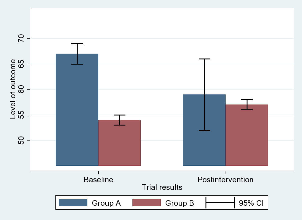
Confidence Intervals: Range of values for which a sample would have if they were to fall close to the mean of the population, with a probability of x%. In other words, you can be x% (normally we use 95%) certain that this range would contain the true mean of the population.
e.g. We calculate CI for 100 times, there should be 95 times that the range calculated would contain the true mean of the population.
Shown as the box-plot lines on bar graphs (example).

5. Z-scores: a way to standardize your data; allow easy comparisions between participants, and between other z-scored measurements; answers the probability of getting a particular value from a normal distribution.

Z distribution has a mean of 0 and SD of 1. “z = -1” means “1 standard deviation away from the mean, in the negative direction”.

1. I added other important ethical issues to the last post (Class #10), including “Vulnerable populations” and “Scientific misconduct”.

2. Types of replication studies:
–Direct replication: Straight from the source; could fail due to the change of the historical background
–Conceptual replication: Re-testing the same theoretical idea using different manipulations
-Replication-plus-extension: Re-testing the original study + adding new variables

3. The Replication Crisis (What might go wrong?)

• Contextually sensitive effects
• Number of replication attempts
• Problems with original study
  • Sample size: Too small
  • Harking: Claiming hypothesis after findings
  • P-hacking: Doing 100,000 analysis, but only reporting the significant results and claiming that’s all they’ve done
• Journals tend to only report new findings but not replication studies

4. What can we do?

• Larger sample sizes
• Report all analyses and variable
• Open Science Collaboration
• Preregistration

1. Researcher’s Obligations: To provide information; to protect the rights and welfare of the participants

2. The Tuskegee Syphilis Study:

• Participants were not treated respectfully
• Participants were harmed
• Participants were targeted, disadvantaged social group

3. The Milgram Obedience Studies:

Lesson: Researchers must balance the risk to participants with benefit to society.

4. The Belmont Report / APA Ethical Principles:

5. Institutional Review Board (IRB): the proposal should descrive the purpose, procedures, and potential risks.

6. Ethical Issues:
-Lack of adequate informed consent
-Invasion of privacy
–Coercion to participate
-Potential physical or mental harm (Minimal Risk)
–Deception
-Violation of confidentiality
–Vulnerable populations (People who have impaied decisional capacity, at risk… e.g., Children, Prisoners…)
-Scientific misconduct (Fabrication, falsification, plagiarism)

7. Informed Consent: Purpose; what the participants will do; possible risks and benefits; statements informing they may refuse to participate with no penalty; confidentiality; encouragement to ask questions; contact information; signature lines for both parties.

1. Economic sample – provides a reasonably accurate estimate of the population at reasonable effort and cost.

2. Things that influence the accuracy of a sample:
-Sample size (the larger, the better)
-Population size (the larger population, the larger sample needed)
-Variance of the data (larger sample size will capture the extreme scores better)

3. Random Samples (Examples):

• Simple Random Sampling: pulling raffle tickets out of a box
• Systematic Random Sampling: randomize the students in our class first, then make every 5th person take an extra exam 🙂
• Stratified Random Sampling:

• Proportionate Random Sampling:

4. Cluster sampling & Multistage clustering

5. Problem of nonresponse: more error.
Solutions: Follow-up with respondents; Incentivize; determine if respondents and nonrespondents differ systematically.

6. Nonprobability Sample

• Convenience Sampling: College students enrolled in Intro to PSY
• Quota Sampling: making sure half of the sample agree with the topic, half disagree
• Purposive Sampling: choosing those who the researcher thinks are most typical of the population

7. Power – the ability of a research design to detect any effects of the variables being studied that exist in the data.
The larger the sample, the higher power.

1. Back to concerns about questionnaires:

• Potential Response Bias – People might tend to answer in a certain way that’ll produce unintended effects.
  • e.g. Social Desirability: In the Burrito Kingdom, every citizen might feel pressured to report that they like burritos.
  • Solutions: Word questions as neutrally as possible; Assure the Ss’ anonymity; Forced-choice approach, items of equal desirability
• Wording – guidelines:
  • Employ objective rather than subjective questions
  • Avoid emotionally charged language
  • Be specific and precise
  • Write the question as simply as possible
  • Avoid difficult words, jargon, phrases
  • Avoid unwarranted assumptions about subjects
  • Conditional Information should precede the question (provide context)
  • No Double Barreled Questions – only ask one questions at a time
  • Choose an appropriate format for your question
  • Pretest your questions

2. Sampling: the process by which a researcher selects participants for a study; how the sample is chosen will determine what can be said about the population
-Sample: A representative group of the population of interest
-Population: Entire group of people interested in studying

3. Probability Sample: the likelihood that any particular individual in the population will be selected for the sample can be identified

4. Representative Sample: we can draw accurate, unbiased estimates of the characteristics of the population 🙂

5. Sampling Error: the extent to which characteristics of individuals selected for the sample differ from those of the population 😦

Error of estimation: indicates the degree to which the data obtained from the sample are expected to deviate from the population
-Effected by: Sample size (the larger, the less error), population size, variance of the data

First of all, CONGRATULATIONS for surviving the first exam! Please do not hesitate to contact Eranda or me if you have any questions about it.

Back to the take-away points:

1. How to test validity?

• Face validity: the extent to which a measure appears to measure what it’s supposed to measure

• Construct Validity: Testing the relationship between the measure of the construct and scores on other measures
  • Convergent Construct Validity: a measure correlates with other measures that it should
  • Discriminant Construct Validity: a measure does not correlate with measures that it should not
• Criterion-Related Validity: Testing how the measure distinguishs among participants on the basis of a particular behavioral criterion (the real world)
  • Concurrent: using two measures at one time
  • Predictive: using a relevant behaviroal criterion at a future time (to test the degree to which those predictions are accurate or useful)

2. Test bias: a particular measure is not equally valid for everyone.
Note: It’s not about how two groups of people score differently. It’s more about when two groups of people should have same scores because they are at the same level on a variable, but they end up scoreing differently because the test has bias.

3. Questionnaires / surveys:

• Self-report: Subject responds about their own feelings or thoughts.
  • Open-Ended Qs: “How do you feel about burritos?”
  • Close-Ended Qs:
    • Fixed Alternative Response Format: “Please choose your feelings about burritos from the following list: love, netural, conflicted, hate.”
    • Rating Scale: “How much do you like burritos?” (1 F-word hate it ~ 5 F-word love it)

4. Concerns about questionnaires:

• Potential Response Bias – People might tend to answer in a certain way that’ll produce unintended effects.
  e.g. Social Desirability: In the Burrito Kingdom, every citizen might feel pressured to report that they like burritos.
• Wording – We’ll talk about this more next week, but using F-word (like I did) in a questionnaire is obviously inappropriate.

1. Measures of Variance:

• Observational
• Physiological
• Self-Report
  Converging operations: Using multiple methods to measure variance

2. Measurement Scales
-Nominal variables
-Continuous variables: Ordinal, Interval, Ratio

3. Observed Score = True score 🙂 + Measurement Error 😦

We want to minimize measurement error, but things happens:

• Transient Participant State (e.g. mood)
• Stable Attributes  (e.g. personality)
• Situational Factors (e.g. noisy environment)
• Characteristics of the Measure (e.g. question in another language)
• Mistakes (e.g. equipment malfunction)

4. Reliability: the consistency or dependability of a measuring technique (e.g. Test-Retest, Inter-item…)
Reliability = True Score Variance / Total Variance
(Higher reliability = lower mesurement error)

5. Validity: The extent to which a measurement procedure measures what it is intended to measure rather than measuring something else (or nothing at all)
e.g. Measuring your own values using random people’s comments: Not valid!

Bonus: A measure can be reliable, but not valid. However, a valid measure is probably reliable.

1. Statistics are everywhere.

2. Numbers don’t mean anything on their own. One definition of statistics is “the process of adding meaning to data”.

3. The shape of data is called their distribution. The classic “bell curve” represents a normal distribution.

4. Statistics places great importance on the presentation of data; visualising statistics helps us to better understand them.

5. The variation of the data is just as important as the average.

Feel the joy of Stats again: https://vimeo.com/18477762

1. The types of studies you choose could affect:

• The way you collect data
• The statistics you use
• The conclusions you can make

2. Psychological science is about looking for and examining systemic behavioral variability. Behavior varies among individuals, changes over time and situations.

3. The Five Factor Model (OCEAN*) explains variability between people, within people and in people across time.
*OCEAN: Openness to experience, Conscientiousness, Extraversion, Agreeableness, Neuroticism

4. Some ways to check variability:

• Range: has limitations, doesn’t tell you anything about middle values
• Variance (s²): the total deviation of the scores around the mean
  • Calculate the mean
  • Subtract the mean from each score
  • Square the deviation scores
  • Add those up for the total sum of squares
  • Divide by n-1
• Standard deviation (√s²): the average deviation of the scores around the mean

5. Total Variance = Systematic Variance 🙂 + Error Variance 😦

1. Science self-corrects by comparing the predictions of a theory with empirical, systematic observations and then adjusts the theory in order to fit the observations.

2. A good theory is parsimonious (simple), testable (falsifiable), and interesting.

3. Types of studies (with examples):

• Descriptive: 77.8% students of our class are female, and…

• Correlational: High attendance rates co-occurs with high grades (True study; Credé, Roch, & Kieszczynka, 2010)
• Experimental: I give money to half of the class, not to the other half, and measure students’ interest in the class (Note: This is a purely hypothetical study)
• Quasi-experimental: Does going to office hours affect your grade? (I can’t control anyone to come to see me, but I can measure)
• Case study: I pick one student from our class, closely analysis his/her attendences, discussions, and behaviors… (Mostly used when there is something particularly unique or rare)

Reference:
Credé, M., Roch, S. G., & Kieszczynka, U. M. (2010). Class attendance in college: A meta-analytic review of the relationship of class attendance with grades and student characteristics. Review of Educational Research, 80(2), 272-295.