1. Generalization mode: Researchers are attempting to make External Validity (this study to the world at large) crutial. That is, to generalize the findings to a population, or other situations. Ecological Validity (lab to the real world) is also important.
The key is to have a representative sample.

2. Theory-testing mode: Researchers are trying to examine some part of a theory. The researchers must have a fair amount of control over the study.
External Validity and Ecological Validity are not as important.

3. Theory Testing using WEIRD samples:
Most research in psychology were conducted on North American college students.

• W – Western
• E – Educated
• I – Industrialized
• R – Rich
• D – Democratic

4. Experimental realism: Laboratory research can just as realistic as research conducted in a field setting.

5. Never forget the role of chance: Our theories can accounts for part of the variability in human behavior, but not all of it!

1. Inflated Type I error: For each test, there’s a α=5% probability that the difference between groups is not meaningful (i.e. due to chance).
If we have n groups to compare, and we keep running t-tests, there will be 1-(1-α)ⁿ chance to make a Type I error!

2. To control for Type I error: Make α smaller; Bonferroni adjustment (divide α by the number of tests). However, Type II error will be larger, power will be lower (more difficult to get a significant result when there is an effect).

3. ANOVA (Analysis of Variance) to-the-rescue: used to analyze more than 2 levels of 1 IV. Answering “Is there any set of means that differs from one another”?

F = Between Groups Variance (Signal) / Within Groups Variance (Noise)
Between Variance = Effect of IV + Individual difference + Error
Within Variance = Individual difference + Error

If H₀ is true (i.e. Effect of IV = 0), then F ≈ 1. The larger the F, the more likely the true effects exist.

4. ANOVA:

• Can stop Type I error inflation while not losing power
• Can tell if there’s significant main effects or interaction
• Can NOT tell which group is causing the difference (one or more of the groups have an effect, but don’t know which)
  • Planned comparisons
  • Post-Hocs

1. When the probability that your results are due to chance/sampling variation is small enough (p <.05), we reject the null, then these results are called statistically significant.
We also mentioned statistically significance during Class #14 Correlation.

2. T-test: tells us the difference between the means of two groups, and an estimate of what differences are expected from sampling variation. –> Whether the observed difference is large enough to be meaningful.

Steps of t-test:
1) The means of the two groups, take the difference
2) The pooled standard deviation, which invloves the standard deviation and sample size for both groups
[Bigger sample size gives us more power.]
3) Use information above to calculate the t score
4) Check the t Table (Morling pg 557) for the Critical Value, based on the degrees of freedom (df = n1+n2-2) and alpha level
5) The critical value is the minimum t score for us to reject the null in this case.
Set α at .05 level, if calculated t > critical t, then p < .05, the probability of getting your result given that the null is true is less than .05, reject null. Conclude that the difference is not caused by chance, but is real.

3. One-tailed t-test and two-tailed t-test: we use a one-tailed t-test when we have a directional hypothesis (X1 > X2), and a two-tailed t-test when we have a non-directional hypothesis (X1 ≠ X2).

When conducting a two-tail test, divide the alpha by 2 for the alpha on each side, then find the critical t.

1. Null Hypothesis (H₀, pronounced as H-nought): The independent variable will not have an effect; there’s no difference between treatment group and control group.
Alternative Hypothesis (H₁): The independent variable has an effect.

When we try to confirm the hypothesis, we are statistically testing the Null Hypothesis. We assume H₀ is true (there is no effect), then we try to prove that the assumption of no effect is very unlikely to happen, to reject the null.

2. Sampling Variation: Even if you have a 50% chance of flipping a coin for heads or tails, you won’t necessarily get 5 heads and 5 tails when you flip a coin 10 times. This is sampling variation. According to a null hypothesis, differences between variables is just this difference.
Theoretically, this possibility can never be excluded. So we can never be 100% sure H₀ is not true. But we can estimate the probability of H₀ being untrue.

3. If we keep drawing random samples of the same size from the same population, we’ll get a normal distribution of the means of the samples.
Greater overlap between null & sample distribution = greater chance of getting results by chance (greater chance of H₀ being true).

4. Inferential statistics are used to answer “How different is different?” – how big of a difference between the means of our conditions we must observe before we conclude that the IV has an effect.

5. The alpha level is the amount of risk the researcher is willing to take to wrongly reject the H₀. (We usually use α = .05)

p-value corresponds to the area of overlap between null distribution and sample distribution.
Image the two distributions completely overlap, then p = 1, accept H₀ with the most confidence.

Therefore, when p <.05, we reject the null. There’s still 5% chance that the difference is caused by chance, so we might have wrongly rejected the H₀, but this is the risk we’re willing to take.
When p>.05, we fail to reject the H₀, because of insufficient evidence to reject.

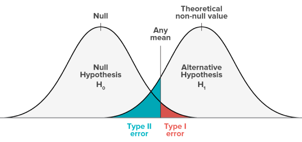
6. Two types of errors:

• Type I error: we reject the null in a case when it is actually true. (We set it to be 5%). — We claim there’s effect when there’s isn’t.
• Type II error: we fail to reject the null even though it is false. — We claim there’s not effect when there’s is.

1. One-way design: manipulating only one independent variable

2. Factorial design: manipulating two or more independent variables
Describing the size and structure of factorial designs:

• 2 × 2 factorial design: 2 IVs; 2 levels for each
• 3 × 3 factorial design: 2 IVs; 3 levels for each
• 2 × 2 × 4 factorial design: 3 IVs; 2 levels, 2 levels, and 4 levels respectively

3. Ways of assigning subjects:

• Randomized groups (between subjects)
• Matched subjects (between subjects)
  • rank order from highest to lowest, divide it into blocks, and then randomly assign subjects from each block to the groups
• Repeated measures (within subjects)
  • reuse the same participants in each condition (to rule out some of the error variance from individual differences)
• Mixed factorial (within & between subjects)
  • some, but not all, independent variables are repeated, participants will be in multiple conditions but not every condition

4. Hypotheses in factorial design
For example, when there are 2 IVs – class size and IQ, and 1 DV – grade:

• Main effect of class size: the difference of grade between large class condition and small class condition
• Main effect of IQ: the difference of grade between high IQ group and low IQ group
• Interaction of class size and IQ: the effect of class size on grade differs between high IQ group and low IQ group; or the effect of IQ on grades differs between large class condition and small class condition

Note: all of the effects above are independent of one another

5. Types of interactions:

• Effect of IV1 is at the same direction for all levels of IV2, but the effect is stronger at one level than at another

• Effect of IV1 at one level of IV2 exists, but not at the other level

• The Crossover – the effect of IV1 goes in different directions for different levels of IV2

1. Again, group designs:

• Randomized Group Design (Between-subjects): each participant is only assigned to ONE condition
• Repeated Measures Design (Within-subjects): each participants gets to be in each condition

2. Repeated Measures (Within-subjects) Design:

• Strengths:
  • Doesn’t need random assignment
  • Has Initial Equivalence (because every subject is the same in each condition)
  • More powerful than Between-subjects design, because it lowers error variance. (i.e. if your hypothesis is correct, more likely to detect the truth)
• Limitations:
  • Order effects: the order of receiving conditions affects behavior (Practice; Fatigue; Sensitization)
  • Solution: Counterbalance or Latin Square Design

3. Counterbalancing: presenting conditions in different orders to different participants, that all possibilities are covered

Latin Square Design: each condition appears once at each ordinal position, each precedes and follows every condition once

4. Carryover Effects: the level of one independent variable are still present when another level of IV is introduced. (E.g., to examine how alcohol affects cognitive ability versus water, give participants 10 glasses of wine in one condition, and give them 10 glasses of water in another. When they are supposed to be tested during the water condition, they are still drunk from the wine condition.)
Some carryovers just can’t be fixed. (E.g., some instructions from condition 1 can not be forgotten during condition 2.)

5. Total variance = treatment [systematic 🙂 ] + confound [systematic 😦 ] + error [unsystematic 😦 ]
Confound variance is hard to distinguished from treatment variance, so it has to be eliminated through experimental design.

6. Experimenter’s Dilemma:

• Internal Validity: the degree to which a researcher draws accurate conclusions about the effects of the IV
  • Some threats:
    • Biased Assignment
    • Attrition (certain types of subject are more likely to drop out)
    • Pretest Sensitization (subjects figure out the hypothesis and change responses accordingly)
    • History (a third, external historical event may affect all participants)
    • Miscellaneous Confounds
  • Threats from beliefs:
    • Experimenter Expectancies
    • Demand Characteristics
    • Placebo Effects
• External Validity: the degree to which the results obtained in one study can be replicated with other samples, research settings, and procedures
• Dilemma: as internal validity increases (tighter control), the external validity decreases (less generalizable)
• Non-issue: experiments are not to be generalized, but to isolate the factors causing behavior. Theories can be generalized through replications, but not a single study.

1. What makes studies experimental?
– Researcher manipulates one variable (the Independent Variable)
– Researcher controls the group assignment (experimental groups + control group [baseline])
– Researcher controls extraneous variables that influnce participants’ behavior (confounds)

2. In experimental studies, we are interested in how one (or more) variable [Independent Variable] changes behavior [Dependent Variable]. NOT just how they are related.
– Independent Variable (IV): the variation (levels) in one variable the researcher set or controlled
– Dependent Variable (DV): response being measured

3. Levels of the IV can vary in two ways (examples):

• Quantitative Differences: make the participants drink 1 cup of beer, 2 cups of beer, or 3 cups of beer (to test how alcohol affects cognitive ability)
• Qualitative Differences: give the participants beer, then tell them to freely choose to drink how much, or tell them most participants in the study chose to drink at least 5 cups (to test the effect of peer pressure on drinking behavior)

4. Ways of manipulating IVs:

• Environmental manipulations: modify the physical or social environment participants are in
• Instructional manipulations: vary the instructions participants receive
• Invasive manipulations: create physical changes in participants’ body
• (Subject variables: existing characteristics of the participants, like Gender; may be treated as manipulation, but not ture IVs)

5. How good is your IV and how can you know?
Good IV: has enough levels to detect changes in behavior.

• Pilot Test (pre-study): measure levels of IV for response
• Manipulation Check (post-study): ensure the levels of IV were effective

6. The assumption of Initially Equivalent: on average, participants didn’t differ in anyway before the IV is given.

Need to randomly assign participants to levels of the IV.
–Simple Random Assignment: every participant has an equal probability to be placed in any condition
–Matched Random Assignment: the conditions will be similar along some specific dimension (e.g. age, intelligence)

7. Group designs:

• Randomized Group Design (Between-subjects): each participant is only assigned to ONE condition
• Repeated Measures Design (Within-subjects): each participants gets to be in each condition

1. Regression analysis: drawing a straight line through the scatter plot, mathematically. Regression analysis can be used to predict the relationship between 2 or more variables.

2. Simple Linear Regression:
y = B₀ + B₁ x 

e.g.: Predicting your grade of PSY310 from the frequency of checking this blog. >:)

3. Multiple Regression Analysis: predicting the outcome variable from more than one predictors.
y = B₀ + B₁x +B₂x +B₃x

Three types:
– Standard Multiple Regression: enter in all predictor variables at once; predicting the outcome variable from all other variables together.
– Stepwise Multiple Regression: enter the predictors one at a time based on the ability to predict the outcome; looking at the unique contributions of individual predictors.
– Hierarchical Multiple Regression: choose order of predictors based on their hypothesis; investigating confounds or mediating variables and possible spurious correlations (controlling for the third variable; whether the chosen new variable uniquely contributes to the variance in the outcome).

4. Output of multiple regressions
Multiple correlation coefficient (R): the degree of relationship between y and a set of x(s). R ranges from 0 to 1.
Coefficient of Multiple Determination (R²): shows the proportion of variance in y that can be accounted for by the set of x(s).
To compare r and R: see post #13.

5. Structural Equation Modeling: hypothesizing how variables are causally related by testing models with directional arrows in them.

1. Interpreting correlations:

Because 1) We don’t know the direction; 2) There could be a third variable involved.

2. Statistical Significance* (p<= .05) for correlation coefficient means: the correlation calculated on the sample has a very low probability of being .00 in the population.
In other words, when p<.05, it’s unlikely that the correlation was not real. Therefore you reject the H0 (i.e. there is no relationship between variable A and B).

3. Cross-Lag Correlations: correlation of the degree to which an earlier measure of one variable is associated with a later measure of the other variable (the bold lines in the picture below).

Cross-lag correlations examines how people change over time.

4. Cross-Lag Four Horsemen: John Gottman used correlations to help understand what lets relationships succeed or fail.
The Four Horseman of the Relationship Apocalypse that he and his colleagues discovered are:

1. Criticism
2. Defensiveness
3. Stonewalling
4. Contempt

1. Correlations answer questions of the relationship between two variables. Scatter plots is one way of determining the form of relationship.

2. Correlation coefficient (r) quantify the linear relationship between two variables.
Pearson r: A statistical index of how 2 variables systematically relate to one another in a linear fashion.

• Range: -1 to +1
• Sign (direction): Positive/Negative
• Magnitude (0-1): the strength of the relationship
  • r =.00 not related at all
  • r =.40 weakly related
  • r = .70 moderately related
  • r =.90 strongly related
  • r = -.90 also strongly related, same magnitude as r = .90

3. Coefficient of Determination (R²): indicates the proportion of variance in one variable that is accounted for by another variable (i.e. the variance shared between variables)
R² = square Pearson’s r, to put the index on a ratio scale
e.g.: 6.25% of the variance is shared between variables with a correlation coefficient of .25

4. Good things about the correlation coefficient (r):
– Quantifies a linear relationship
– Standardizes 2 variables into 1 index
– A single stat tells the direction & strength
– Can be squared to understand in terms of variance

5. Tricky things about the correlation coefficient (r):
– Restricted Range: when the sample includes only a portion of the range of the population, the view of correlation is skewed (e.g., the relationship between the habit of playing video games and happiness will not be accurately found if you only sample people who doesn’t play video games at all. This is extreme, but you get the idea.)
– Outliers: Off-line (deflating the correlation) and On-line (inflating the correlation)

– Reliability: Less reliable a measure is, the lower the correlation (even if there’s a real high correlation in the population)
– Interpretation (see next post)